The Variant Calling Problem
In bioinformatics, particularly in the subfield of oncology in which I work, we're often tasked with the issue of identifying variants
in a genomic sequence. What this means is that we have a sample sequence along with a
reference sequence, and we want to identify
regions where the sample differs from the reference. These regions are called
variants, and they can often be clinically
relevant, potentially indicating an oncogenic mutation or some
other telling clinical marker.
In general, there are two types of variant calling that one may be interested in performing. The first of these is called
germline variant calling. In this type, we use a reference genome that is an accepted standard for the species in
question. There exists more than one acceptable choice for a reference genome, but one of the current standards for humans
is called
GRCh38. This stands for
Genome Reference Consortium human and 38 is an identifying version number.
Note the
h is used to distinguish the human genome from other genomes that the GRC puts out such as
GRCm
(mouse genome).
The second type is called
somatic variant calling. This
method uses two samples from a single individual and compares
the sequence of one with the other. In effect, the patients own
genome serves as the reference. This is the method commonly used
in oncology, as one sample can be taken from a tumor and another
from some non-mutated cell such as the bloodline. This process
is also sometimes called a
tumor-normal study due to the
fact that one sample is taken from the tumor and one from a
normal cell.
There are a few additional things to note in the discussion
above. The first is that in germline calling we're uncovering
variants that are being
passed from parent to child via
the germ cells, i.e. the sperm and eggs. In somatic calling,
we're identifying somatic mutations and variants, those that
occur within the body over the course of a lifetime, whether
they are due to environmental factors, errors in DNA
transcription and translation, or some other factor.
Types of Variants
In order to identify variants, it will be helpful to develop
an ontology of some of the specific classes and types of
variants we might expect to see as the output of our variant
callers.
Indel - This is one of the simplest types of variant
to describe conceptually, but also one of the most difficult
to identify via current variant calling methods. An
indel
is either an insertion or deletion of a single base at some
point in the DNA sequence. The reason these are difficult to
identify is that since it is not known in advance at which
point in the DNA the variant occurs, it can throw off the
alignment with the reference sequence.
SNP - This is short for
single nucleotide polymorphism
and it refers to a population-level variant in which a
single base differs between the sample and reference sequences.
By population-level, we mean that this variant is extremely
common across specific populations. For example, an SNP might
occur when comparing the genomes of Caucasian and Chinese people
within a gene coding for skin tone.
SNV - This stands for
single-nucleotide variant
and is the same as an SNP apart from the fact that it indicates
a novel mutation present in the genomes of a few rather than
being widespread across a population.
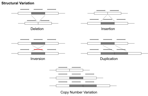
Structural Variant - A
structural variant refers
to a larger-scale variant in the genome, typically occupying at
least 1000 base pairs. These can exhibit a number of different
behaviors. For example, a >1kb region of the DNA can be
duplicated and reinserted or it can be deleted. These types of
structural variation are commonly referred to as
copy number variants (CNVs). A partial sequence can also
be reversed (called
inversion). This image sums it up
well
Haplotype Phasing
Before getting into the nitty gritty of variant calling, it will be helpful to describe a related process called
haplotype phasing. A
haplotype is the set of genetic information associated with a single chromosome.
The human genome is
diploid, meaning it consists of pairs of chromosomes for which each has one part of its genetic information
inherited from the mother and the other part from the father. The combined genetic information resulting from considering these
pairs of chromosomes as single units is called the
genotype. However, having access to the haplotype can be crucial because
it can provide information crucial to identifying disease-causing variants (either SNPs or SNVs) in the genome. The issue is that
current sequencing methods don't give us haplotype information for free as often the reads produced cannot be separated into
their individual male and female loci. Therefore, we need to use statistical algorithms to piece together what we can about the
haplotype sequences after the fact. This is where haplotype phasing comes into play.
Some Preliminaries and Associated Challenges
To start with, we need to establish some background with regards to population-level frequencies of genetic variation so that we
can begin to detect deviations from that standard. What may be surprising is that while the human genome is diploid, it varies
from the reference at approximately 0.1% of the bases. That means that between any two individuals, we should expect to see at
least 99.9% shared genetic information. It is at the remaining 0.1% of sites that we direct our attention when we're looking to
tease out the haplotypes. For reference, the condition of sharing genetic information is often called
homology.
The teasing out of haplotypes is complicated by the fact that at times genetic information is passed from parent to child in a
process known as
recombination. Recombination happens when instead of passing down just one chromosome from its diploid
pair, a parent passes down a combination of the two. At the biological level, this process occurs during
meiosis. The
first phase of meiosis involves an alignment of homologous chromosome pairs between the mother and father. This process involves
a stage in which the chromosomal arms temporarily overlap, causing a crossover which may (or may not) result in fusion at that
locus at which the point of crossover occurs. This results in a recombination of genetic information which is then passed down
to the child. One benefit to this process is that it encourages genetic diversity, creating genetic patterns in the child that
appeared in neither parent. Unfortunately, it also makes haplotype phasing that much more difficult.
DNA sequencing gives partial haplotype information. It produces sequencing
reads which are partial strings of the sequence up to
1000 base pairs. These reads all come from the same chromosome, but they represent only a small slice of the haplotype because the
entire chromosome is on the order of 50 million to 250 million base pairs.
Advantages of Knowing the Haplotype
Hopefully it's clear that having access to the haplotype for any given individual is strictly superior to simply having the genotype.
This is because, given access to a person's haplotype, we can simply combine that information in a procedural way to yield their
genotype. The same cannot be said of the reverse. What's more, having the haplotype allows us to compute statistics about various
biological properties that would otherwise be unavailable to use. For example, if we have haplotypes for a series of individuals
in a population, we can check at which loci recombination is most likely to occur, what the frequency of that recombination is, etc.
It suffices to say that having access to the haplotype is highly advantageous as a downstream input to variant calling methods, and
I'll examine some such methods that make use of this information in upcoming posts.
The DeepVariant Caller
Now that we have an understanding of haplotypes and some of the different ways in which variants might arise, I'd like to introduce
one of the most successful models for variant calling created to-date: Google's
DeepVariant. This model is one of the simplest
to introduce in that it uses virtually no specialized knowledge of genomics in terms of encoding input features. Surprisingly, this
has no detrimental effect on its accuracy, as it outperformed virtually every other variant caller on the market at the time of its
release. The approach it uses is somewhat novel so I'll introduce that here, and I'll compare it in subsequent posts with the
methodology behind other variant callers.
How it Works
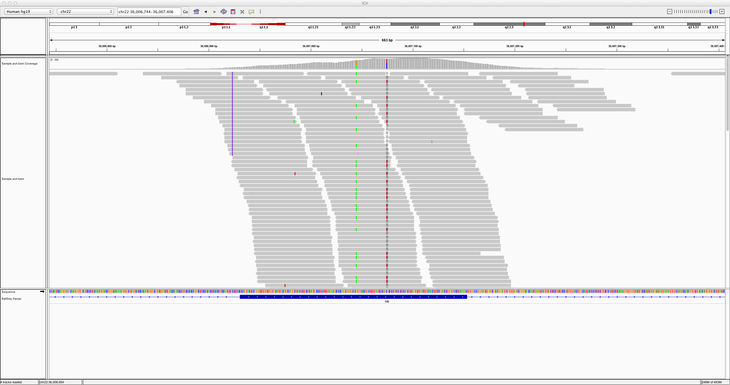
DeepVariant is unique in that it doesn't operate on the textual sequence information of the aligned and reference genomic reads.
Rather, it creates something called a
pileup image from the alignment information. A pileup image shows the sequenced reads from
the sample aligned with the reference. Each base is assigned an RGB color, and possible variants within the reads as compared to the
reference are highlighted accordingly. Here's an example of what a pileup looks like.
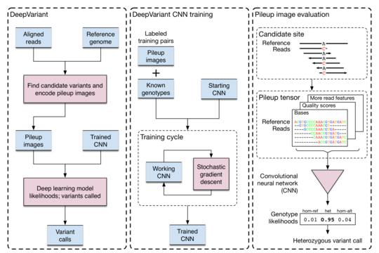
The DeepVariant model is trained on a large dataset of such images in which variants have already been labeled. It can then be applied
to new alignments and samples by generating their pileup using a program such as SAMTOOLS. Here's how the authors from Google
structured their model.
As you can see from the diagram, their workflow proceeds as follows:
- Identifying Candidate Variants and Generating Pileup: Candidate variants are identified according to a simple procedure. The
reads are aligned to the reference, and in each case the CIGAR string for the read is generated. Based on how that read
compares to the reference at the point which it is aligned, it is classified as either a match, an SNV, an insertion, or a
deletion. If the number of reads which differ at that base pass a pre-defined threshold, then that site is identified as a
potential variant. The authors also apply some preprocessing to ensure that the reads under consideration are of high enough
quality and are aligned properly in order to be considered. After candidate variants have been identified, the pileup image is
generated. The notable points here are that candidate variants are colored and areas with excessive coverage are downsampled
prior to image generation.
- The model is trained on the data, then run during inference stages. They use a CNN, specifically the Inception v2 architecture,
which takes in a 299x299 input pileup image and uses an output softmax layer to classify into one of hom-ref, het, or hom-alt.
They use SGD to train with a batch size of 32 and RMS decay set to 0.9. They initialize the CNN to using the weights from one
of the ImageNet models.
The authors find that their model generalizes well, and can be used with no statistically significant loss in accuracy on reads aligned
to a reference different from the one on which
DeepVariant was trained. They also stumble upon another surprising result, namely
that their model successfully calls variants on the mouse genome, opening up the model's to a wide diversity of species.
Conclusion
I hope this post shed some light on how variant calling works and elucidates the biological underpinnings of the process well enough
for newcomers to the field to start diving into some papers. In future posts, I'll expand on some of the other popular variant calling
models as well as introduce algorithms for related processes, such as the haplotype phasing discussed earlier.