Writing Your Own Optimizers in PyTorch
This article will teach you how to write your own optimizers in PyTorch - you know the kind, the ones where you can write something like
optimizer = MySOTAOptimizer(my_model.parameters(), lr=0.001)
for epoch in epochs:
	for batch in epoch:
		outputs = my_model(batch)
		loss  = loss_fn(outputs, true_values)
		loss.backward()
		optimizer.step()
The great thing about PyTorch is that it comes packaged with a great standard library of optimizers that will cover all of your garden variety machine learning needs. However, sometimes you’ll find that you need something just a little more specialized. Maybe you wrote your own optimization algorithm that works particularly well for the type of problem you’re working on, or maybe you’re looking to implement an optimizer from a recently published research paper that hasn’t yet made its way into the PyTorch standard library. No matter. Whatever your particular use case may be, PyTorch allows you to write optimizers quickly and easily, provided you know just a little bit about its internals. Let’s dive in.
Subclassing the PyTorch Optimizer Class
All optimizers in PyTorch need to inherit from torch.optim.Optimizer. This is a base class which handles all general optimization machinery. Within this class,
there are two primary methods that you’ll need to override: __init__ and step. Let’s see how it’s done.
The init Method
The __init__ method is where you’ll set all configuration settings for your
optimizers. Your __init__ method must take a params argument which specifies
an iterable of parameters that will be optimized. This iterable must have a
deterministic ordering - the user of your optimizer shouldn’t pass in something
like a dictionary or a set. Usually a list of torch.Tensor objects is given.
Other typical parameters you’ll specify in the __init__ method include
lr, the learning rate, weight_decays, betas for Adam-based optimizers,
etc.
The __init__ method should also perform some basic checks on passed in
parameters. For example, an exception should be raised if the provided learning
rate is negative.
In addition to params, the Optimizer base class requires a parameter called
defaults on initialization. This should be a dictionary mapping parameter
names to their default values. It can be constructed from the kwarg parameters
collected in your optimizer class’ __init__ method. This will be important in
what follows.
The last step in the __init__ method is a call to the Optimizer base class.
This is performed by calling super() using the following general signature.
super(YourOptimizerName, self).__init__(params, defaults)
Implementing a Novel Optimizer from Scratch
Let’s investigate and reinforce the above methodology using an example taken
from the HuggingFace pytorch-transformers NLP library. They implement a PyTorch
version of a weight decay Adam optimizer from the BERT paper. First we’ll take a
look at the class definition and __init__ method. Here are both combined.
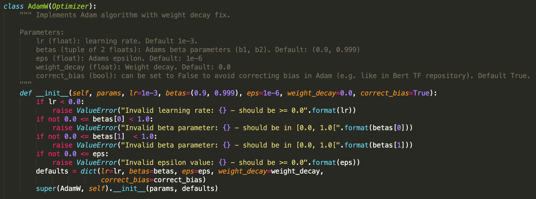
You can see that the __init__ method accomplishes all the basic requirements
listed above. It implements basic checks on the validity of all provided kwargs
and raises exceptions if they are not met. It also constructs a dictionary of
defaults from these required parameters. Finally, the super() method is called
to initialize the Optimizer base class using the provided params and defaults
.
The step() Method
The real magic happens in the step() method. This is where the optimizer’s logic
is implemented and enacted on the provided parameters. Let’s take a look at how
this happens.
The first thing to note in step(self, closure=None) is the presence of the
closure keyword argument. If you consult the PyTorch documentation, you’ll
see that closure is an optional callable that allows you to reevaluate the
loss at multiple time steps. This is unnecessary for most optimizers, but is
used in a few such as Conjugate Gradient and LBFGS. According to the docs,
“the closure should clear the gradients, compute the loss, and return it”.
We’ll leave it at that, since a closure is unnecessary for the AdamW optimizer.
The next thing you’ll notice about the AdamW step function is that it iterates
over something called param_groups. The optimizer’s param_groups is a list
of dictionaries which gives a simple way of breaking a model’s parameters into
separate components for optimization. It allows the trainer of the model to
segment the model parameters into separate units which can then be optimized
at different times and with different settings. One use for multiple param_groups
would be in training separate layers of a network using, for example, different
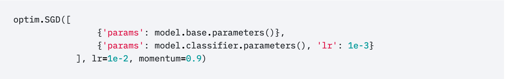
learning rates. Another prominent use cases arises in transfer learning. When
fine-tuning a pretrained network, you may want to gradually unfreeze layers
and add them to the optimization process as finetuning progresses. For this,
param_groups are vital. Here’s an example given in the PyTorch documentation
in which param_groups are specified for SGD in order to separately tune the
different layers of a classifier.
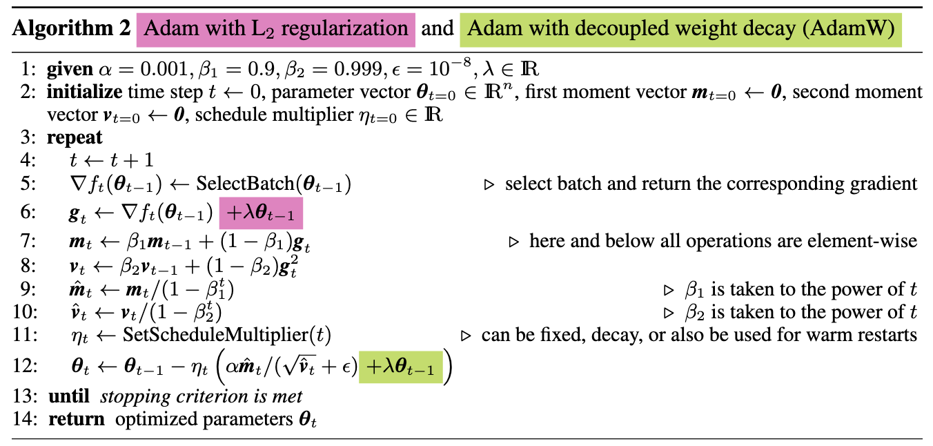
Now that we’ve covered some things specific to the PyTorch internals, let’s get to the algorithm. Here’s a link to the paper which originally proposed the AdamW algorithm. And here, from the paper, is a screenshot of the proposed update rules.
Let’s go through this line by line with the source code. First, we have the loop
for p in group['params']
Nothing mysterious here. For each of our parameter groups, we’re iterating over the parameters within that group. Next.
if p.grad is None:
	continue
grad = p.grad.data
if grad.is_sparse:
	raise RuntimeError('Adam does not support sparse gradients, please consider SparseAdam instead')
This is all simple stuff as well. If there is no gradient for the current
parameter, we just skip it. Next, we get the actual plain Tensor object for
the gradient by accessing p.grad.data. Finally, if the tensor is sparse, we
raise an error because we are not going to consider implementing this for sparse
objects.
Next, we access the current optimizer state with
state = self.state[p]
In PyTorch optimizers, the state is simply a dictionary associated with the
optimizer that holds the current configuration of all parameters.
If this is the first time we’ve accessed the state of a given parameter, then we set the following defaults
if len(state) == 0:
	state['step'] = 0
	# Exponential moving average of gradient values
	state['exp_avg'] = torch.zeros_like(p.data)
	# Exponential moving average of squared gradient values
	state['exp_avg_sq'] = torch.zeros_like(p.data)
We obviously start with step 0, along with zeroed out exponential average and exponential squared average parameters, both the shape of the gradient tensor.
exp_avg, exp_avg_sq = state['exp_avg'], state['exp_avg_sq']
beta1, beta2 = group['betas']

state['step'] += 1
Next, we gather the parameters from the state dict that will be used in the computation of the update. We also increment the current step.
Now, we begin the actual updates. Here’s the code.
# Decay the first and second moment running average coefficient
# In-place operations to update the averages at the same time
exp_avg.mul_(beta1).add_(1.0 - beta1, grad)
exp_avg_sq.mul_(beta2).addcmul_(1.0 - beta2, grad, grad)
denom = exp_avg_sq.sqrt().add_(group['eps'])

step_size = group['lr']
if group['correct_bias']:  # No bias correction for Bert
	bias_correction1 = 1.0 - beta1 ** state['step']
	bias_correction2 = 1.0 - beta2 ** state['step']
	step_size = step_size * math.sqrt(bias_correction2) / bias_correction1

p.data.addcdiv_(-step_size, exp_avg, denom)

# Just adding the square of the weights to the loss function is *not*
# the correct way of using L2 regularization/weight decay with Adam,
# since that will interact with the m and v parameters in strange ways.
#
# Instead we want to decay the weights in a manner that doesn't interact
# with the m/v parameters. This is equivalent to adding the square
# of the weights to the loss with plain (non-momentum) SGD.
# Add weight decay at the end (fixed version)
if group['weight_decay'] > 0.0:
	p.data.add_(-group['lr'] * group['weight_decay'], p.data)
The above code corresponds to equations 6-12 in the algorithm implementation from the paper. Following along with the math should be easy enough. What I’d like to take a closer look at is the built in Tensor methods that allow us to do the in-place computations.
A nice, relatively hidden feature of PyTorch which you might not be aware of is
that you can access any of the standard PyTorch functions, e.g. torch.add(),
torch.mul(), etc. as in-place operations on the Tensors directly by appending
an _ to the method name. Thus, taking a closer look at the first update, we
find we can quickly compute it as
exp_avg.mul_(beta1).add_(1.0 - beta1, grad)
rather than
torch.mul(beta1, torch.add(1.0 - beta1, grad))
Of course, there are a few special operations used here with which you may not
be familiar, for example, Tensor.addcmul_ and Tensor.addcdiv_. This takes the
input and adds it to either the product or dividend, respectively, of the two
latter inputs. If you need a more in-depth rundwon of the various operations
available to be performed on Tensor objects, I highly recommend checking out
this post.
You’ll also see that the learning rate is accessed in the last line in the computation of the final result. This loss is then returned.
And…that’s it! Constructing your own optimizers is as simple as that. Of course, you need to devise your own optimization algorithm first, which can be a little bit trickier ;). I’ll leave that one to you.
Special thanks to the authors of Hugging Face for implementing the AdamW
optimizer in PyTorch.