Differential Privacy –– An Introductory Tutorial

Dec 20, 2025 10 min read Machine Learning, Privacy

In this tutorial, we will:

Implement Laplace and Gaussian mechanisms and explore how ε changes noise.
Apply DP to simple statistics (mean + histogram) and quantify error.
Train a small logistic regression model and add DP via output perturbation.

#@title Setup
import numpy as np
import matplotlib.pyplot as plt

from dataclasses import dataclass
from typing import Tuple, Optional

# For step 3
from sklearn.datasets import make_classification
from sklearn.model_selection import train_test_split
from sklearn.preprocessing import StandardScaler
from sklearn.linear_model import LogisticRegression
from sklearn.metrics import accuracy_score, log_loss

np.random.seed(0)
print("Ready ✅")

Ready ✅

Step 1 — DP Mechanisms (as functions)

We’ll implement two classic DP mechanisms:

Laplace: typically for pure DP (ε-DP) on real-valued queries with L1 sensitivity.
The Laplace mechanism achieves pure differential privacy by adding noise drawn from a Laplace distribution. For a query function $f$ with L1 sensitivity $\Delta_1$ (the maximum change in the query output when a single individual is added/removed), the mechanism releases $f(D) + \text{Lap}(\Delta_1/\epsilon)$, where $\text{Lap}(b)$ denotes a Laplace random variable with scale parameter $b$. The scale is inversely proportional to $\epsilon$: smaller $\epsilon$ (stronger privacy) requires larger noise. This mechanism provides $\epsilon$-DP, meaning the privacy loss is bounded by $\epsilon$ with no failure probability $\delta$. It’s particularly well-suited for queries where the sensitivity is naturally measured in the L1 norm (e.g., counting queries, means of bounded data).
Gaussian: typically for (ε, δ)-DP on real-valued queries with L2 sensitivity.
The Gaussian mechanism achieves approximate differential privacy by adding noise drawn from a Gaussian distribution. For a query function $f$ with L2 sensitivity $\Delta_2$ (the maximum L2-norm change in the query output when a single individual is added/removed), the mechanism releases $f(D) + \mathcal{N}(0, \sigma^2)$, where the variance $\sigma^2$ is calibrated based on $\Delta_2$, $\epsilon$, and a failure probability $\delta$. A common calibration sets $\sigma = \Delta_2 \sqrt{2\ln(1.25/\delta)} / \epsilon$. Unlike the Laplace mechanism, this provides $(\epsilon, \delta)$-DP: the privacy loss exceeds $\epsilon$ with probability at most $\delta$. The Gaussian mechanism is often preferred in practice because Gaussian noise has lighter tails than Laplace noise (better utility for the same privacy), and many machine learning operations naturally work with L2 norms. However, the $(\epsilon, \delta)$ guarantee is slightly weaker than pure $\epsilon$-DP.

#@title DP mechanisms (minimal reference implementations)
def laplace_mechanism(x: float, sensitivity_l1: float, epsilon: float) -> float:
    """Adds Laplace noise calibrated to L1 sensitivity."""
    if epsilon <= 0:
        raise ValueError("epsilon must be > 0")
    scale = sensitivity_l1 / epsilon
    return float(x + np.random.laplace(loc=0.0, scale=scale))

def gaussian_sigma(sensitivity_l2: float, epsilon: float, delta: float) -> float:
    """A common calibration for (ε,δ)-DP Gaussian noise (basic bound).
    """
    if epsilon <= 0:
        raise ValueError("epsilon must be > 0")
    if not (0 < delta < 1):
        raise ValueError("delta must be in (0,1)")
    return float(sensitivity_l2 * np.sqrt(2 * np.log(1.25 / delta)) / epsilon)

def gaussian_mechanism(x: float, sensitivity_l2: float, epsilon: float, delta: float) -> float:
    sigma = gaussian_sigma(sensitivity_l2, epsilon, delta)
    return float(x + np.random.normal(loc=0.0, scale=sigma))

# quick sanity check
print("Laplace sample:", laplace_mechanism(1.0, sensitivity_l1=1.0, epsilon=1.0))
print("Gaussian sample:", gaussian_mechanism(1.0, sensitivity_l2=1.0, epsilon=1.0, delta=1e-5))

Laplace sample: 1.1027273276031648
Gaussian sample: 4.592867568576917

Visualize how ε controls noise

We’ll draw many samples of the noisy answer for different ε and plot the distribution.

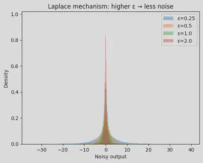
#@title Laplace noise vs epsilon (distribution)
true_x = 0.0
sensitivity = 1.0
epsilons = [0.25, 0.5, 1.0, 2.0]
N = 50_000

plt.figure()
for eps in epsilons:
    samples = np.array([laplace_mechanism(true_x, sensitivity, eps) for _ in range(N)])
    plt.hist(samples, bins=120, density=True, alpha=0.4, label=f"ε={eps}")
plt.title("Laplace mechanism: higher ε → less noise")
plt.xlabel("Noisy output")
plt.ylabel("Density")
plt.legend()
plt.show()

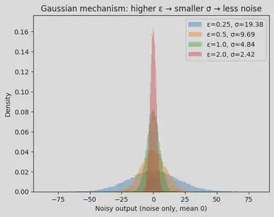
#@title Gaussian noise vs epsilon (distribution)
true_x = 0.0
sensitivity = 1.0
delta = 1e-5
epsilons = [0.25, 0.5, 1.0, 2.0]
N = 50_000

plt.figure()
for eps in epsilons:
    sigma = gaussian_sigma(sensitivity, eps, delta)
    samples = np.random.normal(0.0, sigma, size=N)
    plt.hist(samples, bins=120, density=True, alpha=0.4, label=f"ε={eps}, σ≈{sigma:.2f}")
plt.title("Gaussian mechanism: higher ε → smaller σ → less noise")
plt.xlabel("Noisy output (noise only, mean 0)")
plt.ylabel("Density")
plt.legend()
plt.show()

Quick intuition check

If ε doubles, the noise scale roughly halves.
Bigger sensitivity means bigger noise.

The privacy-utility tradeoff: The parameter $\epsilon$ controls a fundamental tradeoff between privacy and utility. Higher values of $\epsilon$ (e.g., $\epsilon = 5.0$) result in less noise being added, which preserves more utility (accuracy) in the released results. However, this comes at the cost of weaker privacy guarantees—an adversary can learn more about individual data points. Lower values of $\epsilon$ (e.g., $\epsilon = 0.1$) provide stronger privacy protection but require more noise, reducing the utility of the results. In practice, choosing $\epsilon$ involves balancing these competing concerns based on the specific use case, regulatory requirements, and acceptable risk levels. Common values range from $\epsilon = 0.1$ (very strong privacy) to $\epsilon = 10$ (weaker privacy, better utility), though many practitioners aim for $\epsilon \leq 1$ for meaningful privacy protection.

In DP research, a lot of work is about bounding sensitivity or designing a mechanism where sensitivity is low.

Step 2 — DP on simple statistics (mean + histogram)

We’ll create a toy dataset (bounded) and compute DP estimates.

Key idea: Bounded data → bounded sensitivity.

For a mean of data in [0,1], under add/remove neighboring datasets of size n:

L1 sensitivity of the mean is ≤ 1/n.

We’ll compare DP mean to the true mean as ε changes.

#@title Toy bounded dataset
n = 1000
data = np.random.beta(a=2.0, b=5.0, size=n)  # already in [0,1]
true_mean = float(np.mean(data))
print("n =", n)
print("True mean:", true_mean)

n = 1000
True mean: 0.2854443881687054

#@title DP mean experiment (Laplace) — error vs epsilon
def dp_mean_laplace(data: np.ndarray, epsilon: float) -> float:
    n = len(data)
    sensitivity_mean = 1.0 / n  # for data in [0,1]
    return laplace_mechanism(float(np.mean(data)), sensitivity_mean, epsilon)

eps_grid = np.array([0.1, 0.2, 0.5, 1.0, 2.0, 5.0])
trials = 500

errors = []
for eps in eps_grid:
    ests = np.array([dp_mean_laplace(data, eps) for _ in range(trials)])
    mae = float(np.mean(np.abs(ests - true_mean)))
    errors.append(mae)

plt.figure()
plt.plot(eps_grid, errors, marker="o")
plt.xscale("log")
plt.title("DP mean (Laplace): mean absolute error vs ε (log scale)")
plt.xlabel("ε")
plt.ylabel("Mean absolute error")
plt.show()

for eps, mae in zip(eps_grid, errors):
    print(f"ε={eps:<4}  MAE≈{mae:.6f}")

ε=0.1   MAE≈0.010433
ε=0.2   MAE≈0.004696
ε=0.5   MAE≈0.002196
ε=1.0   MAE≈0.000940
ε=2.0   MAE≈0.000492
ε=5.0   MAE≈0.000187

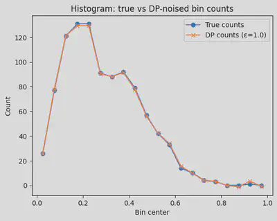
DP Histograms –– Noisy Counts

DP for histograms vs single queries: When we apply DP to a single real-valued query (like the mean), we add noise once using the full privacy budget $\epsilon$. Histograms are different because we’re releasing multiple values (one count per bin). Each bin count has sensitivity 1: adding or removing one individual changes exactly one bin’s count by ±1. However, since we’re releasing all bins simultaneously, we need to account for composition—the privacy cost of releasing multiple statistics.

There are two main approaches: (1) Sequential composition: split the privacy budget $\epsilon$ across all $k$ bins, using $\epsilon/k$ per bin (more conservative, guarantees $\epsilon$-DP overall). (2) Parallel composition: if bins represent disjoint subsets of the data (which they do for histograms), we can use the full $\epsilon$ for each bin and still maintain $\epsilon$-DP overall, since each individual affects only one bin. In practice, the code below adds noise with scale $1/\epsilon$ to each bin independently, which works because histogram bins are disjoint.

We’ll build a histogram and add Laplace noise to each bin count.

#@title DP histogram — noisy counts
def dp_histogram_laplace(data: np.ndarray, bins: int, epsilon: float, data_range=(0.0, 1.0)) -> Tuple[np.ndarray, np.ndarray]:
    counts, edges = np.histogram(data, bins=bins, range=data_range)
    sensitivity = 1.0  # each individual affects exactly one bin by +1
    noisy_counts = np.array([laplace_mechanism(float(c), sensitivity, epsilon) for c in counts])
    return noisy_counts, edges

bins = 20
epsilon = 1.0
noisy_counts, edges = dp_histogram_laplace(data, bins=bins, epsilon=epsilon)

true_counts, _ = np.histogram(data, bins=bins, range=(0,1))
centers = 0.5 * (edges[:-1] + edges[1:])

plt.figure()
plt.plot(centers, true_counts, marker="o", label="True counts")
plt.plot(centers, noisy_counts, marker="x", label=f"DP counts (ε={epsilon})")
plt.title("Histogram: true vs DP-noised bin counts")
plt.xlabel("Bin center")
plt.ylabel("Count")
plt.legend()
plt.show()

Step 3 — DP Logistic Regression via Output Perturbation

Instead of jumping straight into DP-SGD, we’ll:

Train a standard logistic regression model.
Add noise to its learned weights (output perturbation).
Evaluate accuracy and log loss vs ε.

This is not the only DP method for logistic regression, but it’s a great starting point because:

It’s a tiny code footprint.
It makes the privacy–utility tradeoff very visible.

Note: Theoretical DP guarantees for output perturbation typically assume conditions like strong convexity (regularization) and a bounded feature norm. We’ll enforce bounded/standardized features and include L2 regularization.

#@title Generate a small synthetic classification dataset
X, y = make_classification(
    n_samples=5000,
    n_features=20,
    n_informative=10,
    n_redundant=2,
    n_classes=2,
    class_sep=1.0,
    random_state=0,
)

X_train, X_test, y_train, y_test = train_test_split(X, y, test_size=0.25, random_state=0, stratify=y)

scaler = StandardScaler()
X_train = scaler.fit_transform(X_train)
X_test = scaler.transform(X_test)

# Optional: clip feature vectors to a max L2 norm to bound sensitivity-ish behavior
def clip_rows_l2(X: np.ndarray, max_norm: float) -> np.ndarray:
    norms = np.linalg.norm(X, axis=1, keepdims=True) + 1e-12
    factors = np.minimum(1.0, max_norm / norms)
    return X * factors

CLIP_NORM = 5.0
X_train = clip_rows_l2(X_train, CLIP_NORM)
X_test = clip_rows_l2(X_test, CLIP_NORM)

print("Train shape:", X_train.shape, " Test shape:", X_test.shape)

Train shape: (3750, 20)  Test shape: (1250, 20)

#@title Train baseline logistic regression (non-private)
# Stronger regularization helps with DP stability.
C = 1.0  # inverse of regularization strength
base = LogisticRegression(
    penalty="l2",
    C=C,
    solver="lbfgs",
    max_iter=200,
    n_jobs=None
)
base.fit(X_train, y_train)

probs = base.predict_proba(X_test)[:, 1]
preds = (probs >= 0.5).astype(int)

print("Baseline accuracy:", accuracy_score(y_test, preds))
print("Baseline log loss:", log_loss(y_test, probs))

Baseline accuracy: 0.7264
Baseline log loss: 0.5425108769337348

Output perturbation

We’ll add Gaussian noise to the weight vector. We’ll scale noise as σ ∝ 1/ε.

#@title DP via output perturbation — sweep epsilon
w = base.coef_.copy()          # shape (1, d)
b = np.array([base.intercept_[0]])

def predict_with_weights(X: np.ndarray, w: np.ndarray, b: np.ndarray) -> np.ndarray:
    logits = X @ w.T + b  # (n,1)
    logits = logits.reshape(-1)
    return 1.0 / (1.0 + np.exp(-logits))

# Heuristic noise scale: sigma = k / epsilon.
# We'll choose k based on feature clipping and regularization strength to make the tradeoff visible.
# (Not a tight DP calibration; meant for hands-on exploration.)
k = 0.5

eps_grid = np.array([0.2, 0.5, 1.0, 2.0, 5.0])
trials = 30

acc_means, loss_means = [], []
acc_stds, loss_stds = [], []

for eps in eps_grid:
    sigma = k / eps
    accs, losses = [], []
    for _ in range(trials):
        w_noisy = w + np.random.normal(0.0, sigma, size=w.shape)
        b_noisy = b + np.random.normal(0.0, sigma, size=b.shape)

        p = predict_with_weights(X_test, w_noisy, b_noisy)
        yhat = (p >= 0.5).astype(int)

        accs.append(accuracy_score(y_test, yhat))
        losses.append(log_loss(y_test, p))

    acc_means.append(np.mean(accs)); acc_stds.append(np.std(accs))
    loss_means.append(np.mean(losses)); loss_stds.append(np.std(losses))

plt.figure()
plt.errorbar(eps_grid, acc_means, yerr=acc_stds, marker="o")
plt.xscale("log")
plt.title("Output perturbation: accuracy vs ε (log scale)")
plt.xlabel("ε")
plt.ylabel("Accuracy")
plt.show()

plt.figure()
plt.errorbar(eps_grid, loss_means, yerr=loss_stds, marker="o")
plt.xscale("log")
plt.title("Output perturbation: log loss vs ε (log scale)")
plt.xlabel("ε")
plt.ylabel("Log loss")
plt.show()

for eps, am, asd, lm, lsd in zip(eps_grid, acc_means, acc_stds, loss_means, loss_stds):
    print(f"ε={eps:<4}  acc={am:.3f}±{asd:.3f}   loss={lm:.3f}±{lsd:.3f}   (σ={k/eps:.3f})")

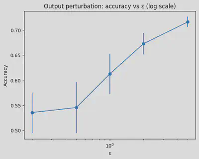
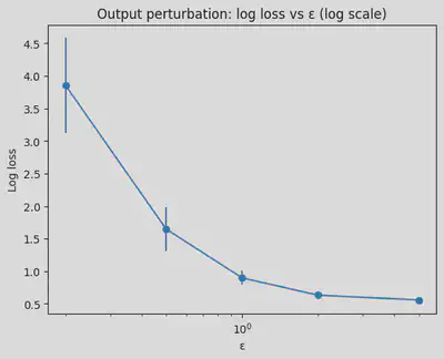
ε=0.2   acc=0.536±0.040   loss=3.852±0.732   (σ=2.500)
ε=0.5   acc=0.545±0.051   loss=1.647±0.335   (σ=1.000)
ε=1.0   acc=0.613±0.040   loss=0.897±0.107   (σ=0.500)
ε=2.0   acc=0.673±0.021   loss=0.632±0.032   (σ=0.250)
ε=5.0   acc=0.716±0.010   loss=0.558±0.009   (σ=0.100)

Interpreting the results

The plots and numerical results above demonstrate the fundamental privacy-utility tradeoff in differential privacy. As $\epsilon$ increases:

Accuracy (utility) increases: With $\epsilon = 0.2$, accuracy is around 0.536, but with $\epsilon = 5.0$, accuracy reaches 0.716—much closer to the baseline non-private accuracy of 0.726. This happens because larger $\epsilon$ values allow less noise to be added (smaller $\sigma = k/\epsilon$), preserving more of the model’s predictive power.
Log loss decreases: Lower log loss indicates better calibrated predictions. The log loss drops from 3.852 at $\epsilon = 0.2$ to 0.558 at $\epsilon = 5.0$, approaching the baseline of 0.543.
Privacy protection decreases: While utility improves, the privacy guarantee weakens. At $\epsilon = 5.0$, an adversary can learn significantly more about individual training examples compared to $\epsilon = 0.2$. The choice of $\epsilon$ represents a deliberate balance: stronger privacy (lower $\epsilon$) comes at the cost of reduced model utility, while better utility (higher $\epsilon$) provides weaker privacy protection.

Notice how the improvement in accuracy is most dramatic when moving from very small $\epsilon$ values (0.2 → 0.5 → 1.0), but the gains diminish as $\epsilon$ increases further. This is a common pattern in DP: there’s often a “sweet spot” where reasonable privacy and utility can coexist, typically in the range $\epsilon \in [0.5, 2.0]$ for many applications.