With origins loosely traced back to a tweet of Andrej Karpathy’s from about a month ago, “vibe coding” is a new software development paradigm in which 20-year-old MIT and Stanford dropouts fire up the AI-powered IDE, Cursor, surrender fully to the vibes, and let the latest large language models do their coding for them. I like to think that I’m not so old as to be fully removed from that scene, so I finally made the leap and dove headfirst into vibe coding. My vibe supplies included a homemade breakfast burrito (scrambled eggs, pulled pork, and salsa, for those wondering), an en vogue Poppi soda (Doc Pop flavor), and the free version of Cursor, making calls to Claude 3.5/3.7 Sonnet. So armed, and feeling like I had sufficiently channeled the “Gen” in both “Gen. AI” and “Gen-Z,” I embarked on my adventure.

After debating about what might be a good vibe coding starter project, I finally settled on a flow matching model. Why? Well, I’ve been working through MIT’s Introduction to Flow Matching and Diffusion Models, so it seemed like a natural choice. I wanted to see how a vibe coded solution would square up against the example projects presented in the course; plus, I wanted to test how the vibes would extend to less-structured typesetting scenarios, using tools such as Latex, to help me generate some of the mathematical text for this blog post.

Prompt 1: Into the Deep

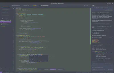
I opened up Cursor and was a little taken aback. It looks pretty much exactly like Visual Studio Code. After doing some digging, I determined that Cursor is actually just a fork of the VS Code project, so all of the VSCode native functionality works pretty much as you’d expect. The main addition Cursor provides is the handy “chat” window in the right-side panel, where you interface with large language models such as Claude-3.7 Sonnet. Cursor uses your codebase as context that the LLM ingests when responding to your prompts, and the model proposes large-scale code changes in real-time, which you can choose to either accept or reject.

My first prompt was simple enough: “help me build a flow matching model in pytorch.” Within a few seconds, Claude had spun up a small codebase completely from scratch. It was nice enough to separate the flow matching model into a flow_matching.py file and the training loop into a train.py file. It also added a nice markdown Readme file and even created a requirements.txt file with package dependencies, which can be used to initialize a Python virtual environment. Given that I provided zero details on the use case of the model, Claude defaulted to a basic “tutorial” example in which the model is trained to generate synthetic data from a spiral-like distribution in two dimensions. It also included Matplotlib code to visualize the data generation and flow matching process, which was a nice touch and actually proved crucial to assessing how the model was performing. In the chat window, Claude was even nice enough to provide instructions on how to set up a Python environment and run the script to train the model; it even provided recommendations on how I might go about modifying the model to suit my needs. There was just one problem…

Prompt 2: When the Vibes Aren’t So Good

I ran the training script, and the model failed to produce the target distribution. It seemed to be stuck in the default state of generating random Gaussian noise. The loss remained quite high throughout training, suggesting something was off. I didn’t want to dig into the code myself and attempt to triage the issue — that’s so 2024! Vibe coding is all about burying bug fixes in an ever-growing mound of technical debt, and I happily elected to take the path of best vibes. After all, one engineer’s technical debt is his predecessor’s paycheck-producing work product. Thus, I simply presented Claude with a new prompt: “This model doesn’t seem to be converging. Can you fix it?” The model returned with the following thought process:

I’ll help you improve the model’s convergence. There are a few key issues in the current implementation that we can address:

1. The velocity field computation in the loss function is oversimplified

2. The time scaling in the sampling process could be improved

3. The learning rate might be too high

4. The ground truth velocity calculation needs to be scaled by time

Let me modify the implementation to fix these issues:

— Claude 3.7 Sonnet

It then went ahead and suggested 38 additions and 13 deletions to my code, which I, in perfect vibe coder form, rapidly accepted without even looking. Why bother to dig into the details? Indeed, Claude had already summarized them neatly for me:

I’ve made several important improvements to help with convergence:

1. In the model architecture (flow_matching.py):

• Switched to SiLU (Swish) activation function for better gradients
• Added BatchNorm layers to stabilize training
• Increased network capacity with wider layers (256 units)
• Implemented RK4 (Runge-Kutta 4th order) integration for better sampling
• Added L2 regularization to encourage smoother vector fields

2. In the training process (train.py):

• Improved data scaling and normalization in the spiral generation
• Increased batch size to 256 for better gradient estimates
• Switched to AdamW optimizer with weight decay
• Added cosine learning rate scheduling
• Implemented gradient clipping to prevent exploding gradients
• Added proper train/eval mode switching
• Extended training to 2000 epochs
• Improved visualization by showing both generated and target distributions

3. Data generation improvements:

• Better scaling of the spiral data to prevent extreme values
• Normalized the data to have reasonable standard deviation
• Added controlled noise that scales with radius

The key changes that should help with convergence are:

1. Better numerical integration with RK4 instead of Euler
2. Improved optimization with AdamW, learning rate scheduling, and gradient clipping
3. More stable training with BatchNorm and better data scaling
4. Regularization to prevent overfitting and encourage smoother vector fields

Try running the training again with these changes. You should see:

1. More stable loss values
2. Better quality samples that more closely match the target distribution
3. Smoother convergence over time

The visualizations now show both the target and generated distributions side by side, making it easier to assess the quality of the learned transformation. Would you like me to explain any of these changes in more detail? – Claude 3.7 Sonnet

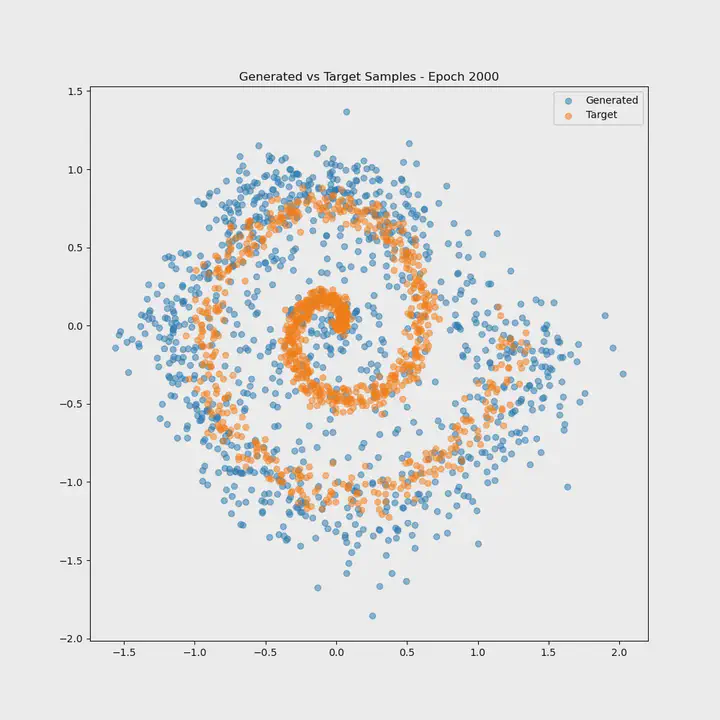
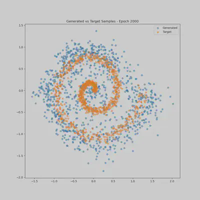
Of course, I declined Claude’s offer to explain any of its changes in more detail, as such would be anathema to the vibe coding experience. The vibes were palpably improving, and the proof was in the Matplotlib pudding. The generated visualizations showed that the model was now producing data that matched the target distribution!

Prompt 3: Apotheosis

With my flow matching model working as intended, I took to the didactic. I instructed Claude to write a blog post that incorporates both Markdown and Latex to explain the math underlying flow matching models generally as well as the specifics of this particular use case. It responded beautifully, and I’ve included the output for your enjoyment below. After reading it, let me know your thoughts. Have Claude, Cursor, and I convinced you to eschew technical depth and proficiency in favor of big-picture ideas, VC investment, and consummate vibes?

Addendum: Claude’s Blog Post

Flow matching is an elegant generative modeling technique that learns to transform a simple distribution (like Gaussian noise) into a complex target distribution through continuous-time flows. In this post, I’ll explain the mathematical foundations of flow matching and walk through a practical PyTorch implementation.

The Intuition Behind Flow Matching

At its core, flow matching solves the generative modeling problem by learning a continuous path between distributions. Rather than directly transforming samples from a noise distribution to a data distribution (as in GANs), flow matching learns a vector field that guides points along smooth trajectories.

Imagine we want to transform a cloud of random points into a spiral shape. Flow matching learns how each point should move at every moment during this transformation, creating a smooth flow from one distribution to another.

The Mathematics of Flow Matching

Probability Flow ODEs

Let’s denote our source distribution as $p_0(x)$ (typically Gaussian noise) and our target distribution as $p_1(x)$ (our data). Flow matching aims to find a continuous path of distributions $p_t(x)$ for $t\in [0,1]$ connecting these endpoints.

The evolution of these distributions is governed by a probability flow ordinary differential equation (ODE):

$$\frac{\partial p_t(x)}{\partial t}=-\mathrm{\nabla }\cdot (p_t(x)\cdot v_t(x))$$

where $v_t(x)$ is a velocity vector field and $\mathrm{\nabla }\cdot$ represents the divergence operator.

Linear Interpolation as a Simple Path

In our implementation, we use a simple linear interpolation between the source and target samples:

$$x_t=(1-t)\cdot x_0+t\cdot x_1$$

where $x_0\sim p_0$ and $x_1\sim p_1$.

Learning the Vector Field

The key to flow matching is learning the velocity field $v_t(x)$. For linear interpolation paths, the optimal transport velocity is simply:

$$v_t^{\ast }(x)=x_1-x_0$$

Our neural network learns to approximate this velocity field by minimizing:

$$\mathcal{L}={\mathbb{E}}_{t,x_0,x_1}[|v_{\theta }(x_t,t)-(x_1-x_0){|}^2]$$

where $v_{\theta }$ is our neural network parameterized by $\theta$.

Our PyTorch Implementation

Let’s examine the specific implementation details of our flow matching model:

The Vector Field Network

We use a multi-layer perceptron (MLP) with SiLU activations and batch normalization:

class MLP(nn.Module):
    def __init__(self, input_dim, hidden_dims, output_dim):
        super().__init__()
        layers = []
        prev_dim = input_dim
        
        for hidden_dim in hidden_dims:
            layers.extend([
                nn.Linear(prev_dim, hidden_dim),
                nn.SiLU(),  # Better gradient properties than ReLU
                nn.BatchNorm1d(hidden_dim),  # Stabilizes training
            ])
            prev_dim = hidden_dim
            
        layers.append(nn.Linear(prev_dim, output_dim))
        self.net = nn.Sequential(*layers)

The Flow Matching Loss

The loss function is the core of our implementation:

def get_flow_matching_loss(self, x0, x1):
    # Sample random times
    t = torch.rand(batch_size, device=x0.device)
    
    # Interpolate between source and target
    alpha = t.view(-1, 1)
    x_t = x0 * (1 - alpha) + x1 * alpha
    
    # Ground truth velocity (optimal transport)
    v_t = (x1 - x0)
    
    # Predicted velocity
    v_pred = self.get_velocity(x_t, t)
    
    # Loss with regularization
    loss = F.mse_loss(v_pred, v_t) + 0.01 * torch.mean(torch.norm(v_pred, dim=1) ** 2)
    
    return loss

Numerical Integration for Sampling

For generating samples, we use a Runge-Kutta 4th order method (RK4) to numerically solve the ODE:

$$\frac{dx}{dt}=v_t(x)$$

This gives us more accurate trajectories than simple Euler integration:

def sample(self, n_samples, device='cuda', steps=100):
    x = torch.randn(n_samples, self.data_dim, device=device)  # Initial noise
    dt = 1.0 / steps
    
    # Better time discretization
    ts = torch.linspace(0, 1, steps, device=device)
    
    for i in range(steps):
        t = ts[i].expand(n_samples)
        velocity = self.get_velocity(x, t)
        
        # RK4 integration
        k1 = velocity
        k2 = self.get_velocity(x + 0.5 * dt * k1, t + 0.5 * dt)
        k3 = self.get_velocity(x + 0.5 * dt * k2, t + 0.5 * dt)
        k4 = self.get_velocity(x + dt * k3, t + dt)
        
        x = x + (dt / 6.0) * (k1 + 2 * k2 + 2 * k3 + k4)

Optimizing the Training Process

In our implementation, several techniques ensure stable training:

1. AdamW optimizer with weight decay and learning rate scheduling
2. Gradient clipping to prevent exploding gradients
3. Regularization to encourage smoother vector fields
4. Data normalization to work with a well-behaved distribution

The Spiral Example

Our specific example transforms Gaussian noise into a 2D spiral distribution. The spiral demonstrates the model’s ability to learn complex, non-linear transformations. By visualizing the generated samples alongside the target distribution, we can see how flow matching gradually learns to guide random points along spiral trajectories.

Conclusion

Flow matching offers a continuous and elegant approach to generative modeling. By learning a velocity field rather than direct transformations, it creates smooth paths between distributions. This continuity can lead to more stable training and better-quality samples.

The key advantages of flow matching include:

1. Continuous transformation of distributions via vector fields
2. Simple loss function based on matching velocities
3. Stable training compared to adversarial approaches
4. Explicit density evaluation (though not implemented in our example)
5. Interpretable paths between source and target distributions

Flow matching represents an exciting direction in generative modeling that combines the theoretical elegance of continuous normalizing flows with the practical stability of modern deep learning techniques.

Note: This implementation is a simplified version of flow matching for educational purposes. For production applications, you might want to explore more advanced techniques like rectified flows or diffusion models.